Chapter 2 - Introduction to Algebra

Groups

Group: a binary operation denoted as * on a set that meets these conditions:

• a * (b*c) = (a*b) * c (associative)
• a*element = element*a = a (has an identity element)
• element_1*element_2 = identity (each member has a pair member that when applied makes the identity element)

Example of a group: XOR on binary numbers (Group = {0,1}, binary operation = XOR, identity elem = 0). Denoted as ⊕. Also called modulo-2 addition.

• Order: the size of the group (e.g. order of binary numbers group is 2)
• finite group: has a fixed, known amount of elements (not infinite)

Fields

Have two elements: addition and multiplication, which meet the following:

• commutative when using +
• Has a zero element for + where a+0=a
• Multiplication with nonzeros is commutative, has a unit element for * where a*1=a
• * is distributive with +: a*(b+c) = a*b + a*c

Like with groups, Order is the size of the field and a finite field has a finite, known number of elements

Prime Fields

• Denoted GF(p) where p is a prime number
• Addition and multiplication are defined as modulo-p addition and multiplication
• E.g. GF(2) uses mod 2 multiplication and mod 2 addition
• Example: GF(7)
  • G = {0,1,2,3,4,5,6}
  • 3 / 2 = 5
    • 3 / 2 = 3 * (2^-1) = 3 * 4 = 5
      • 2^-1 = 4 because (2*4) % 7 = 1 (multiplicative inverse)
      • 3 * 4 = 5 because (3*4) % 7 = 5
  • 3 - 6 = 4
    • 3 - 6 = 3 + (-6) = 3 + 1 = 4
      • -6 = 1 because (6+1) % 7 = 0 (additive inverse)
• Characteristic (λ): the number of increments it takes for the field to loop back to 0. in GF(p) this is always equal to p
  • e.g. λ of GF(7) = 7 because (1+1+1+1+1+1+1) % 7 = 0

Binary Field Arithmetic

Most error coding algs use GF(2) or GF(2^m)

• Uses Modulo 2 addition and multiplication
• Example: solve the set of equations (just like regular algebra)
  • 1) X + Y = 1
  • 2) X + Z = 0
  • 3) X + Y + Z = 1
  • • (X+Y)+Z=1
    • 1+Z=1 -> Z=0 (substitute X+Y in eq 3 with eq 1)
    • X+0=0 -> X=0 (substitute Z in eq 2 with 0)
    • 0+Y+0=1 -> Y=1 (substitute X and Z in eq 3 with 0)
    • X=0, Y=1, Z=0

Binary Field Polynomials

Regular polynomials where there is one variable and its coefficients are either 0 or 1

• Like so: f(X) = f₀ + f₁X + f₂X² + f₃X³ ...
  • where f₀, f₁, ... are 0 or 1
• "A polynomial over GF(2)" means a polynomial with coefficients as 0 or 1

Binary Polynomial Arithmetic

• Addition/subtraction
  • f(X) + g(X) = ((f₀+g₀)%2) + ((f₁+g₁)%2)X + ((f₂+g₂)%2)X² ...
• Multiplication
  • f(X) * g(X) = f₀*g₀ + (f₀*g₁ + f₁*g₀)X + (f₀*g₂ + f₁*g₁ + f₂*g₀)X² ...
    • Where all addition/multiplication is done Modulo 2
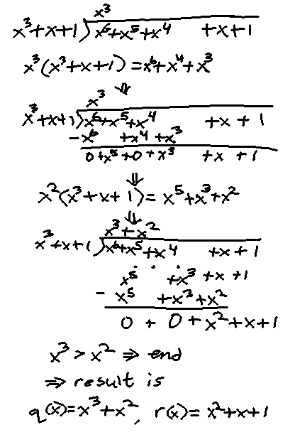
• Division - Euclid's division algorithm
  • given g(X) is NOT 0, f(X)/g(X) = q(X)g(X)+r(X), where q(X) is the quotient and r(X) is the remainder
  • Example: f(X) = 1 + X + X⁴ + X⁵ + X⁶, g(X) = 1 + X + X³

    

Properties of Binary Field Polynomials

• If a is a root of f(X) (f(a)=0), then f(X) is divisible by X-a
• If the polynomial has an even number of terms, it is divisible by X+1
• Irreducible: for f(X) of degree m, f(X) is irreducible if it isn't divisible by any g(X) of degree less than m and greater than 0.
• Any irreducible f(X) of degree m evenly divides X^2m-1 + 1
  • Primitive: an irreducible f(X) is primitive if X^2m-1+1 is the smallest polynomial it divides evenly
• f(X)²ⁱ = f(X²ⁱ) for i >= 0

Galois Field GF(2^m)

Field over GF(2) with 2^m elements as opposed to just 0 and 1

• Field F = {0,1,a,a²,a³,...} with 2^m elements (F finite = {0,1,a,a¹, ...a^2m-2})
• Addition, subtraction, multiplication done Modulo 2 - Notably, when using a:
  • aⁱ * a^j = a^i+j
  • a⁰ = 1
  • aⁱ + a^j = (a_i,0 + a_j,0) + (a_i,1 + a_j,1)a + ... (a_i,m-1 + a_j,m-1) a^m-1 (using modulo 2 addition)
    • 0<= i < 2^m-1
    • a_i(X) = a_i,0 + ... a_i,m-1X^m-1 is the remainder from dividing Xⁱ by p(X)
    • p(X) is primitive with degree m over GF(2), where p(a) = 0 (a is a root of p(X))
    • a^2m-1 = 1 using modulo 2 addition
    • Similarly, a^2m+i loops back around starting at a⁰=1
      • e.g. a¹⁶=a, a¹⁷=a², a¹⁸=a³, etc.
• Example using a within F finite (also denoted F^*)
  • m=4, p(X) = 1+X+X⁴
  • Since a must be a root of p(X), p(a)=1+a+a⁴ = 0
    • 1+a = a⁴ (using mod 2 arith (1 = -1))
  • Use this identity to form the rest of F^*
    • a⁵=a*a⁴=a(1+a)=a+a²
    • a⁶=a*a*a⁴=a²*(1+a)=a²+a³
    • ...
    • a¹⁵ = 1 (last property above (2⁴-1 = 15))
    • So F^* = {0,1,a,a²,a³,a⁴, (a+a²),(a²+a³),...}
• The aⁱ representation makes multiplication easier
  • a⁵*a⁷=a¹²
  • a¹²*a⁷=a¹⁹= a¹⁵*a⁴=1*a⁴=a⁴
• The polynomial representation makes addition easier
  • a⁵+a⁷=(a+a²)+(1+a+a³)=1+(1+1)a+a²+a³ =1+a²+a³=a¹³
• Binary representation makes addition yet again even easier
  • Each bit represents a coefficient in the polynomial, e.g. (1011) = 1+a²+a³
  • Given A=1+a²+a³=(1011), B=1+a²=(1010),
    • A+B = (a₀+b₀)(a₁+b₁)... (a₃+b₃)
    • =(1+1)(0+0)(1+1)(1+0)=(0001)=a³
      • Can be done as a single XOR in C: A^B = (1011)^(1010)=0001

Properties of GF(2^m)

• A polynomial without real roots in GF(2) can have roots in GF(2^m)
  • Ex: X⁴+X³+1 has no roots in GF(2)
  • Plugging in elements from the example GF(2⁴)
  • f(X)=X⁴+X³+1, X=a⁷
    • (a⁷)⁴+(a⁷)³+1
    • a²⁸+a²¹+1
    • a¹³+a⁶+1
    • (1+a²+a³)+(a²+a³) + 1
    • (1101) + (1100) + 1 = (0001) + 1 = 0
  • Hence a⁷ is a root of f(X). The same can be found for a¹¹,a¹³, and a¹⁴
• Conjugate of a polynomial root
  • If B is a polynomial in GF(2^m) and is a root of a polynomial f(X) in GF(2), then B^2l is also a root of f(X) for any l >=0
  • B^2l is a conjugate of B
• Minimal polynomial of B
  • ϕ(X) is the polynomial of the smallest degree where B is a root (ϕ(B)=0), ϕ(X) is in GF(2) and B is in GF(2^m)
  • Example: the minimum polynomial ϕ(X) for B=0 is ϕ(X)=X (since ϕ(B)=0)
  • Example: ϕ(X) for B=1 is ϕ(X)=1+X (since ϕ(B)=1+1=0)

Finding the Minimal Polynomial of B

• ϕ(X) = (X+B²⁰) * (X+B²¹) * ... (X+B^2e-1)
  • Where e is the smallest number so that B^2e=B
  • Example: B=a³ in GF(2⁴)
    • B²=(a³)²=a⁶
    • B⁴=(a³)⁴=a¹²
    • B⁸=(a³)⁸=a²⁴=a⁹
    • ϕ(X) = (X+a³) * (X+a⁶) * (X+a¹²) * (X+a²⁴)
    • which simplifies to ϕ(X) = X⁴ + X³ + X² + X + 1

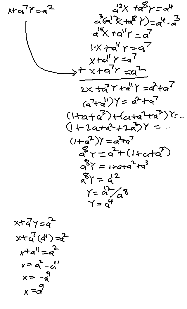
Example Computations Using GF(2^m)

• Solve the linear equations X+a⁷Y = a² and a¹²X + a⁸Y = a⁴ over GF(2⁴)

  • 

  • We can also use Cramer's rule to solve the set of equations (see section 2.6)
• Find the roots of the equation f(X) = X³ + a⁷X + a
  • Can't use quadratic equation because of the divide by 2, and in GF(2), 2=(1+1)=0
  • Instead, plug in and try all of the power representations aⁱ for X and see which ones are roots (f(X) = 0)
    • f(a⁶) = (a⁶)² + (a⁷)(a⁶) + a = a¹² + a¹³ + a = 0
    • f(a¹⁰) = (a¹⁰)² + (a⁷)(a¹⁰) + a = a⁵ + a² + a = 0
• The above two previous examples are used in BCH and Reed-Solomon coding

Vector Spaces

Vector space over GF(2)

• n-tuple over GF(2): (a₀,a₁,a₂,a₃...a_n-1) where a₀...a_n-1 are in GF(2) (equal 0 or 1)
• V_n = the set of all possible n-tuples (2ⁿ possible tuples)
• for n-tuples u and v,
  • u + v = (u₀ + v₀, u₁ + v₁, ...)
    • Where addition is Modulo 2
  • v+v=0 (since 1+1=0)
  • The additive inverse of v (-v) is v itself
• Scalar multiplication: a*v = (a*v₀,a*v₁,...)
  • Multiplication is Modulo 2
• Linear combination: a₁v₁ + a₂v₂ + ... a_kv_k
  a_1...k and v_1...k are k scalars and vectors from vector space V and field F

Matrices

A k by n matrix G over GF(2) has k rows and n columns, where each entry is in GF(2) (0 or 1)

• Matrix can also be represented by its k rows, where each row is a n-tuple vector
• Row space: If the k rows (assuming k <= n) are linearly independant, then any linear combination of these rows called the row space of G
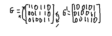
• Elementary row operations: Adding or swapping any of these rows is valid and is called a elementary row operation

  

• Adding matrices:
  • The number of rows and cols must be the same
  • Uses scalar addition: A+B=C, where C_i,j = A_i,j+B_i,j
• Multiplying matrices:
  • Number of cols in A must equal the number of rows in B
  • Each entry in result is the dot product/inner product of the row in A and col in B